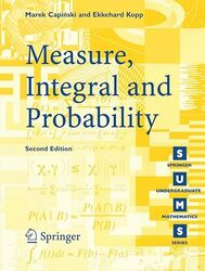
Rating: 7.8/10.
A textbook on measure theory, which serves as the foundation of probability and also has applications to integration and mathematical finance. A measure essentially defines the length or area of a set in a formal and consistent way, even with infinite sets that arise in continuous probability. When defined in a naive way, this can lead to various paradoxes with very specific constructions involving the axiom of choice, leading to nonmeasurable sets. Therefore, the theory must be constructed rigorously to exclude any possibility of paradoxes using unusual constructions.
Many of the concepts and proofs proceed as follows: a finite version of the theorem is proven first, which is straightforward using elementary techniques. Then, some machinery is introduced to transition from finite cases to the infinite case using some kind of limit theorem, such as the monotone convergence theorem. The property is then proven in the infinite case and serves as a foundation to build out various probability concepts.
I found that this book is quite rigorous but relatively lacking in intuitive explanations. It focuses on rigorous and detailed proofs, so I needed to find other resources to gain the intuition necessary to understand what is going on. The final sections of each chapter is a section on the probability applications, followed by some mathematical finance applications of the theory developed in the chapter. I skipped the sections on mathematical finance because the book does not adequately explain these concepts for readers who are not already familiar with finance.
Chapter 1. Begins with a review of set theory, countable sets, topology of the reals (open sets and limits). The Riemann integral has some serious limitations when dealing with infinite domains, infinite points of discontinuity, and lacks convergence of the integral of the limit of functions (for limits of integrals to converge, a stronger notion of uniform convergence is required, as a sequence of continuous functions may not be continuous or integrable). Generally, simpler theories of probability only work well for finite objects but break down when handling infinity, such as an infinite set of events, the union of infinitely many sets, etc, so more advanced theories are needed.
Chapter 2. A null set, intuitively having zero length, is such that for any epsilon > 0, we can cover it with intervals whose total length is less than epsilon. Any countable set is null, and some unmeasurable sets are as well, like the Cantor set, which is defined by recursively removing one-third of the intervals. We can define the length of an interval [a,b] as b-a, and the outer measure is the tightest covering (infimum) of a set by intervals. It satisfies some intuitive properties, such as the outer measure of an interval being equal to its length and the outer measure of a union being less than or equal to the sum of the outer measures (countable subadditivity). The former property is nontrivial to prove, mainly proving the impossibility of a union of sets with measure less than 1 to cover the interval [0, 1] requires some real analysis, such as the Heine-Borel theorem. A set is Lebesgue-measurable if its outer measure can be defined and satisfies a bunch of additivity properties. A sigma field gives a natural family of Lebesgue measurable sets, defined by starting with intervals and allowing countable unions and intersections of sets that are in the sigma field.
Some properties of Lebesgue measure: the Lebesgue measure of any set may be approximated closely by a sequence of open sets. The Borel field is the smallest sigma field that contains all intervals, and it does not make a difference whether we use open or closed intervals since it leads to the same field. The Borel field is smaller than the set of all measurable sets (for a measurable set that is not Borel, a construction based on the Cantor set can be done); for every measurable set, we can find a larger Borel set with the same measure. The theory of measure can be used as a framework for probability; given a sigma field of events and probability measure such that the P(empty set) = 0 and P(event space) = 1, we can define concepts like conditional probability, independence, etc.
Chapter 3. Measurable Functions. A function is said to satisfy some property almost surely or almost everywhere if the set of points where it does not satisfy the property is a null set. Lebesgue integration, instead of splitting up the domain, splits up the range and then considers the inverse images of range intervals. These images will not be intervals, but if the function is measurable, then the inverse image sets will be measurable, and the function can be integrated. Measurable functions include all continuous functions and are closed under addition, multiplication, and limits. Changing the function arbitrarily on a null set maintains its Lebesgue integral. A random variable is a function from a set of outcomes to a real number; assume that sets are always Borel, and the sigma field generated by a random variable consists of all possible inverse images of the function, representing the information produced by the random variable.
Chapter 4: Lebesgue Integration splits the range of a function into intervals, and for each interval, we obtain an upper and lower sum similar to Riemann integrals, multiplying by the measure of the inverse image. There are several possible definitions that are equivalent: it is possible to approximate a function from below using simple functions (functions that have finitely many range values and all inverse images are measurable). This equivalent definition is useful since it allows one to work with simple functions whose integrals are finite sums.
Fatou’s Lemma states that the lim inf of a sequence of integrals is greater than the integral of the pointwise lim inf of functions. The Monotone Convergence Theorem is if a sequence of functions increases monotonically and converges pointwise to f, then the limit of the integrals also converges to the integral of f. The space of Lebesgue integrable functions over a measure satisfies the properties of a vector space, such as additivity and scalar multiplication. The dominated convergence theorem is similar to MCT, but applies to a sequence of functions fn that converge pointwise to a function f: if |f| < g where g is some integrable function then the limit of the integral of the sequence fn is the integral of f. Beppo Levi’s theorem allows the rearrangement of an infinite sum of a function, to swap the order of summation and integration.
The Riemann integral exists only if the function is continuous almost everywhere, and when the Riemann integral exists, it is the same as the Lebesgue integral; however, an improper Riemann integral may exist without the function being Lebesgue integrable, eg, in cases where the function oscillates between positive and negative values: Lebesgue integration requires both the positive and negative parts of the function to be integrable, and the difference is taken to be the Lebesgue integral. In the case of non-negative functions the existence of an improper Riemann integral implies that the Lebesgue integral is equal.
This concept can be applied to probability density functions, which must integrate over the sample space to 1. The cumulative distribution function (CDF) integrates from -inf to a point, and a continuous cumulative distribution function does not always imply that a density function exists (counterexample is the Cantor distribution); the existence of a density function requires the stronger condition of absolute continuity. There are 3 conditions for a function to be a CDF of a random variable: it must be non-decreasing, its limit at -inf is 0 and its limit at inf is 1, and it must be right-continuous to handle the case of discrete points. The chapter ends with the definition of the expectation and characteristic function of a random variable.
Chapter 5. The space of Lebesgue integrable functions, L^1, is a metric space with a norm where the distance is defined by the integral. It defines an equivalence class where functions that only differ on a null set are considered equivalent. The L^1 space is complete, so every Cauchy sequence converges to something in the space. The Hilbert space L^2 consists of functions whose squares are integrable and has similar properties of being a metric space with normal properties and is complete. An inner product space has an inner product operation that satisfies additional properties, such as the parallelogram law, and the only L^p space that is an inner product space is L^2; no other L^p space can satisfy the inner product laws. In an inner product space, we can define the angle between vectors, and orthogonal projection is well defined.
L^p spaces are functions where the pth powers are integrable, and the norm can be defined so that they are complete, but there is no inner product. Hölder’s inequality is a generalization of Cauchy-Schwarz to multiple dimensions, and Minkowski’s inequality is a generalization of the triangle inequality. These are used to prove that the norm satisfies the required properties in L^p spaces to be a normed metric space. For L^inf, a norm is defined as the essential supremum (kind of like the maximum where null sets are ignored). The space L^p gets smaller as p gets larger.
L^p spaces are relevant to probability because the expectation of X^k is the kth moment. The first moment is the mean, the second is the variance, and central moments are the expectation of centered random variables (can be determined from regular moments and vice versa). Not all densities have moments, like the Cauchy distribution. The independence of random variables can be defined by whether the integral of arbitrary functions of them can be decoupled into the product of separate parts. Conditional expectation can be defined by taking a sub-sigma-field G of F and then finding an orthogonal projection of a random variable X onto G (can be thought of as best approximation of F within G). It can then be shown that the expectation of X on G is unique and is the conditional expectation.
Chapter 6. A product sigma-field generalizes to multiple dimensions by taking the product of Borel sets or intervals. A product measure is defined by integrating over the cross-section of one dimension, and it can be proven that any section of a 2D measurable set is always 1D measurable. A product measure is unique and is determined by its values on rectangles – the proof involves the monotone class theorem to generalize results from rectangles to more general sets. Fubini’s theorem says integral over a 2D measure can be transformed into iterated integral of one dimension at a time. Product measures are useful for defining joint distributions of random variables, and they are independent if the joint density is the product of the individual densities. Fubini’s theorem also allows us to define conditional expectation in terms of integrals and slices of the joint density function. Finally, it is proven that the characteristic function uniquely determines the density of a distribution using the inversion formula.
Chapter 7. This chapter is probably the most dense and technical of the whole book, and I skipped some sections. A measure ν is absolutely continuous wrt μ if, whenever μ assigns zero measure to a set, then ν also assigns zero measure, and we write ν << μ. The Radon-Nikodym theorem states that whenever ν << μ, there is always a unique function h such that integrating this function over μ gives ν. We then call h the Radon-Nikodym derivative, denoted h = dν/dμ. The proof of this theorem begins with the simplified case of nu dominated by mu and uses simple functions h before taking a limit for the general case. In probability, mu is usually the whole Lebesgue measure, and h is essentially a density function derived from the measure nu.
The Lebesgue-Stieltjes measure: given a right-continuous monotonic function F, we can construct a measure from it, called the F-outer measure. This is similar to the outer measure that assigns a value to sets, but instead of taking the length of intervals b – a, we take the difference evaluated at F, so F(b) – F(a). This essentially constructs a measure from a CDF function. The two theorems relate measure and density function, showing how they are constructed from each other, similar to the fundamental theorem of calculus. An application to probability is conditional expectation: the Radon-Nikodym theorem provides a construction of conditional expectation that is more general than the version from Chapter 5, which relies on the existence of orthogonal projections that only hold for L^2 space.
Chapter 8. The final chapter is about limit theorems, which are useful in statistics. Convergence of a sequence of functions: strongest is uniform convergence, which implies pointwise convergence, which in turn implies convergence almost everywhere (pointwise convergence except on a null set). Convergence in the L^p norm is neither stronger nor weaker than the other three. Convergence of sequence of random variables, convergence in probability is weaker than convergence almost surely. The weak law of large numbers (LLN) states that the mean of i.i.d. random variables converges in L^2 to the mean (variance goes to zero), this implies convergence in probability; the easiest version assumes finite variance since this can be proved using Chebyshev’s inequality and does not require stronger tools. Other versions can be proven under weaker conditions about tail behavior than finite variance. The LLN can be useful for many applications, such as proving the convergence of a function approximated by Bernstein polynomials.
The Borel-Cantelli lemma is about how many times a ‘bad’ event can occur in an infinite sequence of events: if the total probability converges to a finite number, then the probability it occurs infinitely many times is 0; conversely, if the total probability is infinite, then the probability it occurs infinitely many times is 1. What follows are several versions of the strong law of large numbers, which state that the mean of i.i.d. random variables converges almost surely. The most general form does not require finite moments, only that the mean is finite; the proof starts with strong conditions on moments and gradually relaxes these conditions until no such condition is needed anymore. Finite mean is necessary because if the mean is not finite, then there are cases where the LLN does not hold.
Weak convergence is if the CDF converges at all points where the CDF is continuous, and convergence in probability implies the CDF weakly converges. However, the Skorokhod representation theorem says that if the CDF converges weakly, then there exist corresponding random variables that converge almost surely, and also the characteristic functions converge. Lévy’s theorem states that if the characteristic functions converge, then this implies that the CDF distribution weakly converges. Finally, the last theorem and the longest proof in the book is the Lindeberg-Feller central limit theorem, which states that for a sequence of random variables, if they are independent and each one has finite expectation and variance, then the sum converges to the Gaussian distribution with the given mean and variance.


